第十六讲:投影矩阵和最小二乘
上一讲中,我们知道了投影矩阵\(P=A(A^TA)^{-1}A^T\),\(Pb\)将会把向量投影在\(A\)的列空间中。
举两个极端的例子: * 如果\(b\in C(A)\),则\(Pb=b\); * 如果\(b\bot C(A)\),则\(Pb=0\)。
一般情况下,\(b\)将会有一个垂直于\(A\)的分量,有一个在\(A\)列空间中的分量,投影的作用就是去掉垂直分量而保留列空间中的分量。
在第一个极端情况中,如果\(b\in C(A)\)则有\(b=Ax\)。带入投影矩阵\(p=Pb=A(A^TA)^{-1}A^TAx=Ax\),得证。
在第二个极端情况中,如果\(b\bot C(A)\)则有\(b\in N(A^T)\),即\(A^Tb=0\)。则\(p=Pb=A(A^TA)^{-1}A^Tb=0\),得证。
向量\(b\)投影后,有\(b=e+p, p=Pb, e=(I-P)b\),这里的\(p\)是\(b\)在\(C(A)\)中的分量,而\(e\)是\(b\)在\(N(A^T)\)中的分量。
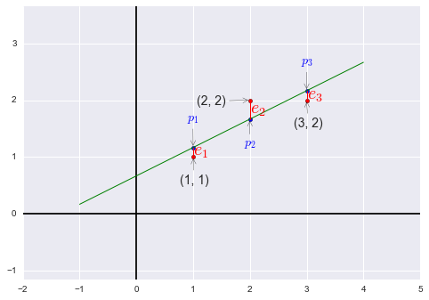
回到上一讲最后提到的例题:
我们需要找到距离图中三个点 \((1, 1), (2, 2), (3, 2)\) 偏差最小的直线:\(y=C+Dt\)。
%matplotlib inline
import matplotlib.pyplot as plt
from sklearn import linear_model
import numpy as np
import pandas as pd
import seaborn as sns

x = np.array([1, 2, 3]).reshape((-1,1))
y = np.array([1, 2, 2]).reshape((-1,1))
predict_line = np.array([-1, 4]).reshape((-1,1))

regr = linear_model.LinearRegression()
regr.fit(x, y)
ey = regr.predict(x)

fig = plt.figure()
plt.axis('equal')
plt.axhline(y=0, c='black')
plt.axvline(x=0, c='black')

plt.scatter(x, y, c='r')
plt.scatter(x, regr.predict(x), s=20, c='b')
plt.plot(predict_line, regr.predict(predict_line), c='g', lw='1')
[ plt.plot([x[i], x[i]], [y[i], ey[i]], 'r', lw='1') for i in range(len(x))]

plt.annotate('(1, 1)', xy=(1, 1), xytext=(-15, -30), textcoords='offset points', size=14, arrowprops=dict(arrowstyle="->"))
plt.annotate('(2, 2)', xy=(2, 2), xytext=(-60, -5), textcoords='offset points', size=14, arrowprops=dict(arrowstyle="->"))
plt.annotate('(3, 2)', xy=(3, 2), xytext=(-15, -30), textcoords='offset points', size=14, arrowprops=dict(arrowstyle="->"))

plt.annotate('$e_1$', color='r', xy=(1, 1), xytext=(0, 2), textcoords='offset points', size=20)
plt.annotate('$e_2$', color='r', xy=(2, 2), xytext=(0, -15), textcoords='offset points', size=20)
plt.annotate('$e_3$', color='r', xy=(3, 2), xytext=(0, 1), textcoords='offset points', size=20)

plt.annotate('$p_1$', xy=(1, 7/6), color='b', xytext=(-7, 30), textcoords='offset points', size=14, arrowprops=dict(arrowstyle="->"))
plt.annotate('$p_2$', xy=(2, 5/3), color='b', xytext=(-7, -30), textcoords='offset points', size=14, arrowprops=dict(arrowstyle="->"))
plt.annotate('$p_3$', xy=(3, 13/6), color='b', xytext=(-7, 30), textcoords='offset points', size=14, arrowprops=dict(arrowstyle="->"))
plt.draw()
plt.close(fig)
根据条件可以得到方程组 $ \begin{cases} C+D&=1 \ C+2D&=2 \ C+3D&=2 \ \end{cases} \(,写作矩阵形式 \(\begin{bmatrix}1&1 \\1&2 \\1&3\\\end{bmatrix}\begin{bmatrix}C\\D\\\end{bmatrix}=\begin{bmatrix}1\\2\\2\\\end{bmatrix}\),也就是我们的\)Ax=b$,很明显方程组无解。
我们需要在\(b\)的三个分量上都增加某个误差\(e\),使得三点能够共线,同时使得\(e_1^2+e_2^2+e_3^2\)最小,找到拥有最小平方和的解(即最小二乘),即\(\left\|Ax-b\right\|^2=\left\|e\right\|^2\)最小。此时向量\(b\)变为向量\(p=\begin{bmatrix}p_1\\p_2\\p_3\end{bmatrix}\\\)(在方程组有解的情况下,\(Ax-b=0\),即\(b\)在\(A\)的列空间中,误差\(e\)为零。)我们现在做的运算也称作线性回归(linear regression),使用误差的平方和作为测量总误差的标准。
注:如果有另一个点,如\((0, 100)\),在本例中该点明显距离别的点很远,最小二乘将很容易被离群的点影响,通常使用最小二乘时会去掉明显离群的点。
现在我们尝试解出\(\hat x=\begin{bmatrix}\hat C\\ \hat D\end{bmatrix}\)与\(p=\begin{bmatrix}p_1\\p_2\\p_3\end{bmatrix}\)。
写作方程形式为\(\begin{cases}3\hat C+16\hat D&=5\\6\hat C+14\hat D&=11\\\end{cases}\),也称作正规方程组(normal equations)。
回顾前面提到的“使得误差最小”的条件,\(e_1^2+e_2^2+e_3^2=(C+D-1)^2+(C+2D-2)^2+(C+3D-2)^2\),使该式取最小值,如果使用微积分方法,则需要对该式的两个变量\(C, D\)分别求偏导数,再令求得的偏导式为零即可,正是我们刚才求得的正规方程组。(正规方程组中的第一个方程是对\(C\)求偏导的结果,第二个方程式对\(D\)求偏导的结果,无论使用哪一种方法都会得到这个方程组。)
解方程得\(\hat C=\frac{2}{3}, \hat D=\frac{1}{2}\),则“最佳直线”为\(y=\frac{2}{3}+\frac{1}{2}t\),带回原方程组解得\(p_1=\frac{7}{6}, p_2=\frac{5}{3}, p_3=\frac{13}{6}\),即\(e_1=-\frac{1}{6}, e_2=\frac{1}{3}, e_3=-\frac{1}{6}\)
于是我们得到\(p=\begin{bmatrix}\frac{7}{6}\\\frac{5}{3}\\\frac{13}{6}\end{bmatrix}, e=\begin{bmatrix}-\frac{1}{6}\\\frac{1}{3}\\-\frac{1}{6}\end{bmatrix}\),易看出\(b=p+e\),同时我们发现\(p\cdot e=0\)即\(p\bot e\)。
误差向量\(e\)不仅垂直于投影向量\(p\),它同时垂直于列空间,如 \(\begin{bmatrix}1\\1\\1\end{bmatrix}, \begin{bmatrix}1\\2\\3\end{bmatrix}\)。
接下来我们观察\(A^TA\),如果\(A\)的各列线性无关,求证\(A^TA\)是可逆矩阵。
先假设\(A^TAx=0\),两边同时乘以\(x^T\)有\(x^TA^TAx=0\),即\((Ax)^T(Ax)=0\)。一个矩阵乘其转置结果为零,则这个矩阵也必须为零(\((Ax)^T(Ax)\)相当于\(Ax\)长度的平方)。则\(Ax=0\),结合题设中的“\(A\)的各列线性无关”,可知\(x=0\),也就是\(A^TA\)的零空间中有且只有零向量,得证。
我们再来看一种线性无关的特殊情况:互相垂直的单位向量一定是线性无关的。
- 比如\(\begin{bmatrix}1\\0\\0\end{bmatrix}\begin{bmatrix}0\\1\\0\end{bmatrix}\begin{bmatrix}0\\0\\1\end{bmatrix}\),这三个正交单位向量也称作标准正交向量组(orthonormal vectors)。
- 另一个例子\(\begin{bmatrix}\cos\theta\\\sin\theta\end{bmatrix}\begin{bmatrix}-\sin\theta\\\cos\theta\end{bmatrix}\)
下一讲研究标准正交向量组。
