4.3 – RNN 循环神经网络 (回归 Regression)
循环神经网络让神经网络有了记忆, 对于序列话的数据,循环神经网络能达到更好的效果. 如果你对循环神经网络还没有特别了解, 请观看几分钟的短动画,RNN 动画简介(如下) 和 LSTM(如下)动画简介 能让你生动理解 RNN. 上次我们提到了用 RNN 的最后一个时间点输出来判断之前看到的图片属于哪一类, 这次我们来真的了, 用 RNN 来及时预测时间序列.
RNN 简介
LSTM 简介
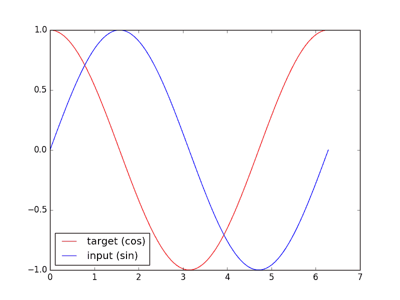
训练数据
我们要用到的数据就是这样的一些数据, 我们想要用 sin 的曲线预测出 cos 的曲线.
import torch
from torch import nn
from torch.autograd import Variable
import numpy as np
import matplotlib.pyplot as plt

torch.manual_seed(1)    # reproducible

# Hyper Parameters
TIME_STEP = 10      # rnn time step / image height
INPUT_SIZE = 1      # rnn input size / image width
LR = 0.02           # learning rate
DOWNLOAD_MNIST = False  # set to True if haven\'t download the data
RNN模型
这一次的 RNN, 我们对每一个 r_out 都得放到 Linear 中去计算出预测的 output , 所以我们能用一个 for loop 来循环计算. 这点是 Tensorflow 望尘莫及的! 除了这点, 还有一些动态的过程都可以在这个教程中查看, 看看我们的 PyTorch 和 Tensorflow 到底哪家强.
class RNN(nn.Module):
    def __init__(self):
        super(RNN, self).__init__()

        self.rnn = nn.RNN(  # 这回一个普通的 RNN 就能胜任
            input_size=1,
            hidden_size=32,     # rnn hidden unit
            num_layers=1,       # 有几层 RNN layers
            batch_first=True,   # input & output 会是以 batch size 为第一维度的特征集 e.g. (batch, time_step, input_size)
        )
        self.out = nn.Linear(32, 1)

    def forward(self, x, h_state):  # 因为 hidden state 是连续的, 所以我们要一直传递这一个 state
        # x (batch, time_step, input_size)
        # h_state (n_layers, batch, hidden_size)
        # r_out (batch, time_step, output_size)
        r_out, h_state = self.rnn(x, h_state)   # h_state 也要作为 RNN 的一个输入

        outs = []    # 保存所有时间点的预测值
        for time_step in range(r_out.size(1)):    # 对每一个时间点计算 output
            outs.append(self.out(r_out[:, time_step, :]))
        return torch.stack(outs, dim=1), h_state

rnn = RNN()
print(rnn)
"""
RNN (
  (rnn): RNN(1, 32, batch_first=True)
  (out): Linear (32 -> 1)
)
"""
其实熟悉 RNN 的朋友应该知道, forward 过程中的对每个时间点求输出还有一招使得计算量比较小的. 不过上面的内容主要是为了呈现 PyTorch 在动态构图上的优势, 所以我用了一个 for loop 来搭建那套输出系统. 下面介绍一个替换方式. 使用 reshape 的方式整批计算.
def forward(self, x, h_state):
    r_out, h_state = self.rnn(x, h_state)
    r_out_reshaped = r_out.view(-1, HIDDEN_SIZE) # to 2D data
    outs = self.linear_layer(r_out_reshaped)
    outs = outs.view(-1, TIME_STEP, INPUT_SIZE)  # to 3D data
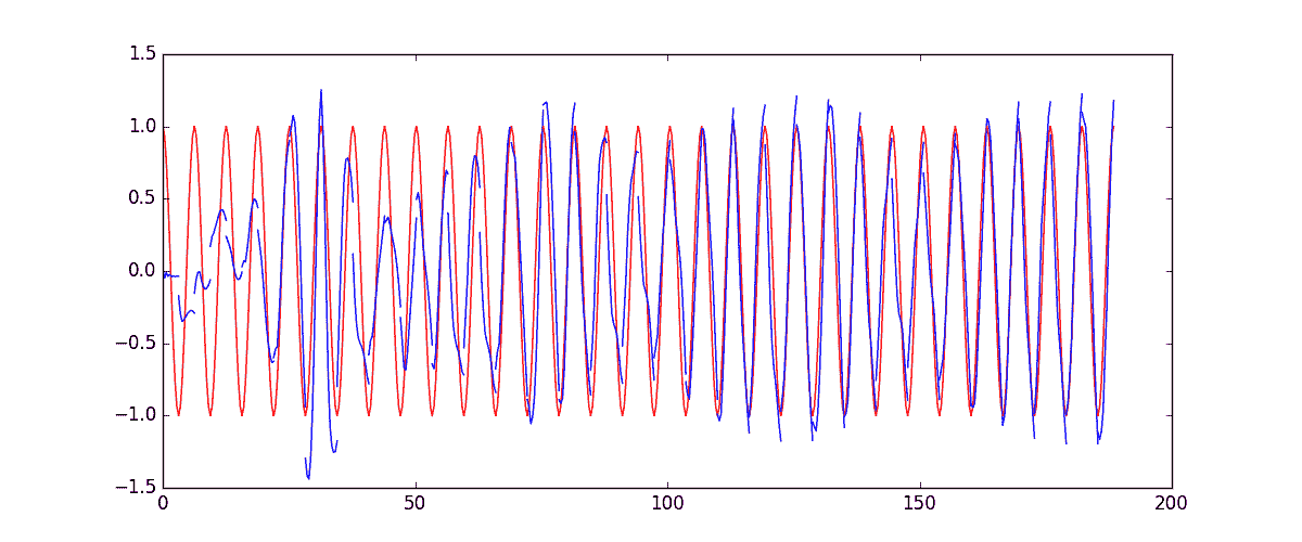
训练
下面的代码就能实现动图的效果啦~开心, 可以看出, 我们使用 x 作为输入的 sin 值, 然后 y作为想要拟合的输出, cos 值. 因为他们两条曲线是存在某种关系的, 所以我们就能用 sin 来预测 cos. rnn 会理解他们的关系, 并用里面的参数分析出来这个时刻 sin 曲线上的点如何对应上 cos 曲线上的点.
optimizer = torch.optim.Adam(rnn.parameters(), lr=LR)   # optimize all rnn parameters
loss_func = nn.MSELoss()

h_state = None   # 要使用初始 hidden state, 可以设成 None

for step in range(60):
    start, end = step * np.pi, (step 1)*np.pi   # time steps
    # sin 预测 cos
    steps = np.linspace(start, end, 10, dtype=np.float32)
    x_np = np.sin(steps)    # float32 for converting torch FloatTensor
    y_np = np.cos(steps)

    x = Variable(torch.from_numpy(x_np[np.newaxis, :, np.newaxis]))    # shape (batch, time_step, input_size)
    y = Variable(torch.from_numpy(y_np[np.newaxis, :, np.newaxis]))

    prediction, h_state = rnn(x, h_state)   # rnn 对于每个 step 的 prediction, 还有最后一个 step 的 h_state
    # !!  下一步十分重要 !!
    h_state = Variable(h_state.data)  # 要把 h_state 重新包装一下才能放入下一个 iteration, 不然会报错

    loss = loss_func(prediction, y)     # cross entropy loss
    optimizer.zero_grad()               # clear gradients for this training step
    loss.backward()                     # backpropagation, compute gradients
    optimizer.step()                    # apply gradients
所以这也就是在我 github 代码 中的每一步的意义啦.
文章来源:莫烦
