4.2 – RNN 循环神经网络 (分类 Classification)
循环神经网络让神经网络有了记忆, 对于序列话的数据,循环神经网络能达到更好的效果. 如果你对循环神经网络还没有特别了解, 请观看几分钟的短动画, RNN 动画简介(如下) 和 LSTM(如下) 动画简介 能让你生动理解 RNN. 接着我们就一步一步做一个分析手写数字的 RNN 吧.
RNN 简介
LSTM 简介
MNIST手写数据
import torch
from torch import nn
from torch.autograd import Variable
import torchvision.datasets as dsets
import torchvision.transforms as transforms
import matplotlib.pyplot as plt

torch.manual_seed(1)    # reproducible

# Hyper Parameters
EPOCH = 1           # 训练整批数据多少次, 为了节约时间, 我们只训练一次
BATCH_SIZE = 64
TIME_STEP = 28      # rnn 时间步数 / 图片高度
INPUT_SIZE = 28     # rnn 每步输入值 / 图片每行像素
LR = 0.01           # learning rate
DOWNLOAD_MNIST = True  # 如果你已经下载好了mnist数据就写上 Fasle

# Mnist 手写数字
train_data = torchvision.datasets.MNIST(
    root=\\'./mnist/\\',    # 保存或者提取位置
    train=True,  # this is training data
    transform=torchvision.transforms.ToTensor(),    # 转换 PIL.Image or numpy.ndarray 成
                                                    # torch.FloatTensor (C x H x W), 训练的时候 normalize 成 [0.0, 1.0] 区间
    download=DOWNLOAD_MNIST,          # 没下载就下载, 下载了就不用再下了
)
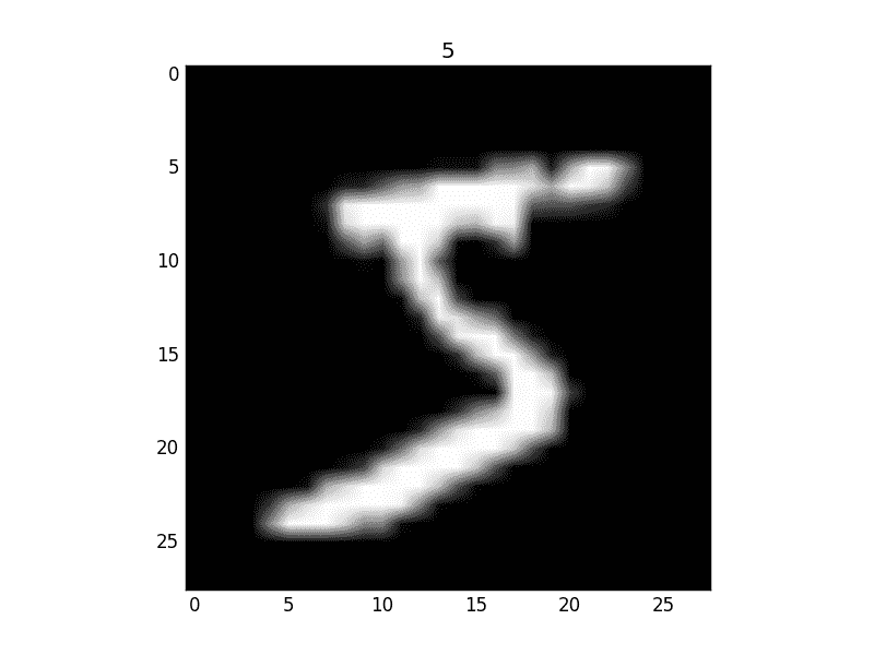
黑色的地方的值都是0, 白色的地方值大于0.
同样, 我们除了训练数据, 还给一些测试数据, 测试看看它有没有训练好.
test_data = torchvision.datasets.MNIST(root=\\'./mnist/\\', train=False)

# 批训练 50samples, 1 channel, 28x28 (50, 1, 28, 28)
train_loader = Data.DataLoader(dataset=train_data, batch_size=BATCH_SIZE, shuffle=True)

# 为了节约时间, 我们测试时只测试前2000个
test_x = Variable(torch.unsqueeze(test_data.test_data, dim=1), volatile=True).type(torch.FloatTensor)[:2000]/255\.   # shape from (2000, 28, 28) to (2000, 1, 28, 28), value in range(0,1)
test_y = test_data.test_labels[:2000]
RNN模型
和以前一样, 我们用一个 class 来建立 RNN 模型. 这个 RNN 整体流程是
- (input0, state0) -> LSTM -> (output0, state1) ;
- (input1, state1) -> LSTM -> (output1, state2) ;
- …
- (inputN, stateN)-> LSTM -> (outputN, stateN 1) ;
- outputN -> Linear -> prediction . 通过LSTM分析每一时刻的值, 并且将这一时刻和前面时刻的理解合并在一起, 生成当前时刻对前面数据的理解或记忆. 传递这种理解给下一时刻分析.
class RNN(nn.Module):
    def __init__(self):
        super(RNN, self).__init__()

        self.rnn = nn.LSTM(     # LSTM 效果要比 nn.RNN() 好多了
            input_size=28,      # 图片每行的数据像素点
            hidden_size=64,     # rnn hidden unit
            num_layers=1,       # 有几层 RNN layers
            batch_first=True,   # input & output 会是以 batch size 为第一维度的特征集 e.g. (batch, time_step, input_size)
        )

        self.out = nn.Linear(64, 10)    # 输出层

    def forward(self, x):
        # x shape (batch, time_step, input_size)
        # r_out shape (batch, time_step, output_size)
        # h_n shape (n_layers, batch, hidden_size)   LSTM 有两个 hidden states, h_n 是分线, h_c 是主线
        # h_c shape (n_layers, batch, hidden_size)
        r_out, (h_n, h_c) = self.rnn(x, None)   # None 表示 hidden state 会用全0的 state

        # 选取最后一个时间点的 r_out 输出
        # 这里 r_out[:, -1, :] 的值也是 h_n 的值
        out = self.out(r_out[:, -1, :])
        return out

rnn = RNN()
print(rnn)
"""
RNN (
  (rnn): LSTM(28, 64, batch_first=True)
  (out): Linear (64 -> 10)
)
"""
训练
我们将图片数据看成一个时间上的连续数据, 每一行的像素点都是这个时刻的输入, 读完整张图片就是从上而下的读完了每行的像素点. 然后我们就可以拿出 RNN 在最后一步的分析值判断图片是哪一类了. 下面的代码省略了计算 accuracy 的部分, 你可以在我的 github 中看到全部代码.
optimizer = torch.optim.Adam(rnn.parameters(), lr=LR)   # optimize all parameters
loss_func = nn.CrossEntropyLoss()   # the target label is not one-hotted

# training and testing
for epoch in range(EPOCH):
    for step, (x, y) in enumerate(train_loader):   # gives batch data
        b_x = Variable(x.view(-1, 28, 28))   # reshape x to (batch, time_step, input_size)
        b_y = Variable(y)   # batch y

        output = rnn(b_x)               # rnn output
        loss = loss_func(output, b_y)   # cross entropy loss
        optimizer.zero_grad()           # clear gradients for this training step
        loss.backward()                 # backpropagation, compute gradients
        optimizer.step()                # apply gradients
"""
...
Epoch:  0 | train loss: 0.0945 | test accuracy: 0.94
Epoch:  0 | train loss: 0.0984 | test accuracy: 0.94
Epoch:  0 | train loss: 0.0332 | test accuracy: 0.95
Epoch:  0 | train loss: 0.1868 | test accuracy: 0.96
"""
最后我们再来取10个数据, 看看预测的值到底对不对:
test_output = rnn(test_x[:10].view(-1, 28, 28))
pred_y = torch.max(test_output, 1)[1].data.numpy().squeeze()
print(pred_y, \\'prediction number\\')
print(test_y[:10], \\'real number\\')
"""
[7 2 1 0 4 1 4 9 5 9] prediction number
[7 2 1 0 4 1 4 9 5 9] real number
"""
所以这也就是在我 github 代码 中的每一步的意义啦.
文章来源:莫烦
