4.1 – CNN 卷积神经网络
卷积神经网络目前被广泛地用在图片识别上, 已经有层出不穷的应用, 如果你对卷积神经网络还没有特别了解, 我制作的 卷积神经网络 动画简介 (如下) 能让你花几分钟就了解什么是卷积神经网络. 接着我们就一步一步做一个分析手写数字的 CNN 吧.
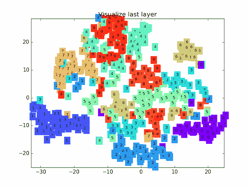
下面是一个 CNN 最后一层的学习过程, 我们先可视化看看:
MNIST手写数据
import torch
import torch.nn as nn
from torch.autograd import Variable
import torch.utils.data as Data
import torchvision      # 数据库模块
import matplotlib.pyplot as plt

torch.manual_seed(1)    # reproducible

# Hyper Parameters
EPOCH = 1           # 训练整批数据多少次, 为了节约时间, 我们只训练一次
BATCH_SIZE = 50
LR = 0.001          # 学习率
DOWNLOAD_MNIST = True  # 如果你已经下载好了mnist数据就写上 Fasle

# Mnist 手写数字
train_data = torchvision.datasets.MNIST(
    root=\\'./mnist/\\',    # 保存或者提取位置
    train=True,  # this is training data
    transform=torchvision.transforms.ToTensor(),    # 转换 PIL.Image or numpy.ndarray 成
                                                    # torch.FloatTensor (C x H x W), 训练的时候 normalize 成 [0.0, 1.0] 区间
    download=DOWNLOAD_MNIST,          # 没下载就下载, 下载了就不用再下了
)
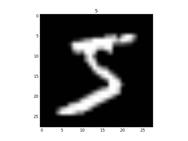
黑色的地方的值都是0, 白色的地方值大于0.
同样, 我们除了训练数据, 还给一些测试数据, 测试看看它有没有训练好.
test_data = torchvision.datasets.MNIST(root=\\'./mnist/\\', train=False)

# 批训练 50samples, 1 channel, 28x28 (50, 1, 28, 28)
train_loader = Data.DataLoader(dataset=train_data, batch_size=BATCH_SIZE, shuffle=True)

# 为了节约时间, 我们测试时只测试前2000个
test_x = Variable(torch.unsqueeze(test_data.test_data, dim=1), volatile=True).type(torch.FloatTensor)[:2000]/255\.   # shape from (2000, 28, 28) to (2000, 1, 28, 28), value in range(0,1)
test_y = test_data.test_labels[:2000]
CNN模型
和以前一样, 我们用一个 class 来建立 CNN 模型. 这个 CNN 整体流程是 卷积( Conv2d ) -> 激励函数( ReLU ) -> 池化, 向下采样 ( MaxPooling ) -> 再来一遍 -> 展平多维的卷积成的特征图 -> 接入全连接层 ( Linear ) -> 输出
class CNN(nn.Module):
    def __init__(self):
        super(CNN, self).__init__()
        self.conv1 = nn.Sequential(  # input shape (1, 28, 28)
            nn.Conv2d(
                in_channels=1,      # input height
                out_channels=16,    # n_filters
                kernel_size=5,      # filter size
                stride=1,           # filter movement/step
                padding=2,      # 如果想要 con2d 出来的图片长宽没有变化, padding=(kernel_size-1)/2 当 stride=1
            ),      # output shape (16, 28, 28)
            nn.ReLU(),    # activation
            nn.MaxPool2d(kernel_size=2),    # 在 2x2 空间里向下采样, output shape (16, 14, 14)
        )
        self.conv2 = nn.Sequential(  # input shape (1, 28, 28)
            nn.Conv2d(16, 32, 5, 1, 2),  # output shape (32, 14, 14)
            nn.ReLU(),  # activation
            nn.MaxPool2d(2),  # output shape (32, 7, 7)
        )
        self.out = nn.Linear(32 * 7 * 7, 10)   # fully connected layer, output 10 classes

    def forward(self, x):
        x = self.conv1(x)
        x = self.conv2(x)
        x = x.view(x.size(0), -1)   # 展平多维的卷积图成 (batch_size, 32 * 7 * 7)
        output = self.out(x)
        return output

cnn = CNN()
print(cnn)  # net architecture
"""
CNN (
  (conv1): Sequential (
    (0): Conv2d(1, 16, kernel_size=(5, 5), stride=(1, 1), padding=(2, 2))
    (1): ReLU ()
    (2): MaxPool2d (size=(2, 2), stride=(2, 2), dilation=(1, 1))
  )
  (conv2): Sequential (
    (0): Conv2d(16, 32, kernel_size=(5, 5), stride=(1, 1), padding=(2, 2))
    (1): ReLU ()
    (2): MaxPool2d (size=(2, 2), stride=(2, 2), dilation=(1, 1))
  )
  (out): Linear (1568 -> 10)
)
"""
训练
下面我们开始训练, 将 y 都用 Variable 包起来, 然后放入 cnn 中计算 output, 最后再计算误差. 下面代码省略了计算精确度 accuracy 的部分, 如果想细看 accuracy 代码的同学, 请去往我的 github 看全部代码.
optimizer = torch.optim.Adam(cnn.parameters(), lr=LR)   # optimize all cnn parameters
loss_func = nn.CrossEntropyLoss()   # the target label is not one-hotted

# training and testing
for epoch in range(EPOCH):
    for step, (x, y) in enumerate(train_loader):   # 分配 batch data, normalize x when iterate train_loader
        b_x = Variable(x)   # batch x
        b_y = Variable(y)   # batch y

        output = cnn(b_x)               # cnn output
        loss = loss_func(output, b_y)   # cross entropy loss
        optimizer.zero_grad()           # clear gradients for this training step
        loss.backward()                 # backpropagation, compute gradients
        optimizer.step()                # apply gradients

"""
...
Epoch:  0 | train loss: 0.0306 | test accuracy: 0.97
Epoch:  0 | train loss: 0.0147 | test accuracy: 0.98
Epoch:  0 | train loss: 0.0427 | test accuracy: 0.98
Epoch:  0 | train loss: 0.0078 | test accuracy: 0.98
"""
最后我们再来取10个数据, 看看预测的值到底对不对:
test_output = cnn(test_x[:10])
pred_y = torch.max(test_output, 1)[1].data.numpy().squeeze()
print(pred_y, \\'prediction number\\')
print(test_y[:10].numpy(), \\'real number\\')

"""
[7 2 1 0 4 1 4 9 5 9] prediction number
[7 2 1 0 4 1 4 9 5 9] real number
"""
可视化训练(视频中没有)
这是做完视频后突然想要补充的内容, 因为可视化可以帮助理解, 所以还是有必要提一下. 可视化的代码主要是用 matplotlib 和 sklearn 来完成的, 因为其中我们用到了 T-SNE 的降维手段, 将高维的 CNN 最后一层输出结果可视化, 也就是 CNN forward 代码中的 x = x.view(x.size(0), -1) 这一个结果.
可视化的代码不是重点, 我们就直接展示可视化的结果吧.
所以这也就是在我 github 代码 中的每一步的意义啦.
文章来源:莫烦
